CHE 341 Lab 1 Lesson

Background Part 2: Spectroscopy and the Bradford Assay

Suggested Reading

• Wilson and Walker 13.1 - 13.1.2 and 13.2-13.2.4.

Lecture Video

Reagent Blanks in Spectrophotometry

Beer's Law lets you calculate the concentration of a substance in solution after measuring the absorbance with a spectrophotometer. Before using a spectrophotometer, it must be properly calibrated, or zeroed. If it is not, the values generated will be meaningless.

One problem often encountered in spectrophotometry is that an absorbance is present at a given wavelength not due to the substance of interest. We handle that by mixing up a reagent blank, which is a control in which everything is included except the substance for which we are testing. The absorbance of the reagent blank is then subtracted from the other readings.

This week we want to read the absorbance at 595 nm of a protein solution mixed with a colorizing bye solution called Bradford reagent. What is a suitable reagent blank? We should mix everything that might contribute to an absorbance at 595 nm except the protein we are trying to measure. Therefore, the best reagent blank is a tube of the dye (Bradford reagent) without any added protein. By zeroing the instrument on this tube, the absorbance due to the Bradford reagent is subtracted out automatically. 

The Limits of Spectrophotometry

Spectrophotometry is frequently used to determine the concentration of a light-absorbing compound present in a solution. Beer's Law, A = ε×l×c, states that the absorption (A) of a given compound at constant conditions is related to a unique extinction coefficient (ε, also known as the molar absorptivity coefficient) of the compound, the concentration of the compound (c), and the length of the light path (l). Provided that you know the extinction coefficient of a particular compound, you can then use the above equation to determine the concentration of the compound by measuring its absorbance. Similarly, you can predict the absorbance that will be observed for any concentration of the compound.

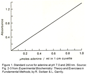
Regardless of the method used, Beer's Law dictates that spectrophotometric quantification of an analyte requires a known relationship between its absorbance and concentration. In many experiments, the extinction coefficient is invariable and Beer's Law may be used. This linear relationship can be demonstrated using adenine. As the adenine concentration is increased, the absorbance increases proportionately, see Figure 1.¹ The linear Beer's Law equation may be used to for measurement of the concentration of an unknown sample from absorbance.

However, colorometric assays involve the development of a color that corresponds to an extinction coefficient that may change with time or is sensitive to interfering compounds in matrix of the solution. For such experiments, we must record the response of a set of standards with known concentrations in order to generate the absorbance-concentration relationship. This is called generating a standard curve.

In standard curves the linear relationship between concentration and absorbance becomes nonlinear at high concentrations of the compound of interest, see Figure 2a. This is typically due to the fact molecules near the light source can cast shadows on molecules further from the light source at high concentration. Thus, not all molecules have the opportunity to encounter the incident light, see Figure 2b. The non-linearity of spectrophotometry is especially significant for color-forming reactions on the surface of large analytes, like the methods we will use this week. Additional sources of non-linearity at high concentration include saturation of the colorant related to the analyte (due to shortages of the colorant caused by interfering compounds in the solution) and variations in the concentration of unreacted dye across the measured range.

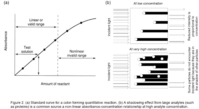
All measured values that fall in the nonlinear region of the curve must be omitted since the concentration of the compound cannot be accurately calculated from these assays. The measurement must be rerun using less of the compound of interest, in an attempt to obtain absorbance values in the linear region of the curve. Most investigators initially assay a wide range of amounts of the compound with the hope that one or more values will fall within the linear or valid quantitative photometry range indicated by a standard curve. A standard curve is a plot of A versus a varying known amount of a substance. The unknown concentration can be determined from the graph, see Test solution in Figure 2a.

When using a color-forming reaction, the need to prepare a standard curve is doubly important because the color intensity is dependent on many factors such as development time of the reaction and freshness of the reagents. Although Beer's Law dictates that there is a linear relationship between absorbance and concentration, the effective extinction coefficient commonly varies with each experiment. Therefore, it is essential to make a standard curve using generic proteins of known concentration and determine the concentration of our unknown by graphing.

 

Example of a Standard Curve

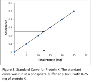
We have a compound X of varying concentrations in a phosphate buffer, pH 7.0, and measure the following absorbances. What is the concentration of an unknown sample of X with an absorbance of 0.30?

 

First, you must understand corrected absorbance. Tube 1 has an absorbance of 0.05, but it does not contain any of the compound that we are measuring. This tube is our reagent blank, yet it has an absorbance. In Beers Law, if c = 0, then A must also equal 0. Therefore, the graph must have a curve that goes through zero. There are two ways of dealing with this. The first way is to subtract the absorbance (0.05) from all the absorbances. This gives the data shown in the last column. The second way is to zero the spectrophotometer with tube 1. That way, the subtraction is done automatically. I suggest you always use corrected curves even though the difference between a corrected curve and an uncorrected one is essentially cosmetic. Continuing with the example, first subtract the reagent blank (tube 1) from the rest to give the corrected absorbance; then plot Absorbance versus corrected concentration (see graph below). On the graph, look for the Absorbance that corresponds to the unknown, 0.30 - 0.05 (blank) = 0.25. This corresponds to 12.5 mg of X in the unknown sample. Information on how to construct standard curves in Excel and how to perform data analysis with them is given in the Data Analysis section of this lesson. This will be necessary for completing the post-lab assignment.

It is important to note that the absorbance value of your unknown must fall within the line of your standard curve. Extrapolating your line beyond your highest concentration is never permitted!

I have found that a major source of frustration for many students is figuring out just what to plot against absorbance for these types of experiments. Two quantities can be plotted. Many students are tempted to plot final concentration of their protein after adding the test solution. However, the final concentration in your reaction assay is not important. What we care about is the amount of protein added to each reaction. As long as you treat every assay reaction the same way, you can plot amount of protein against absorbance, as in the example above.

Bradford Assay

An assay is an analytical procedure in biochemistry, laboratory medicine, and related molecular and cell biology fields for qualitatively assessing or quantitatively measuring the presence, amount, or functional activity of a target entity (called an analyte) typically in a blood, cell, tissue, or even whole organism sample. The analyte is most commonly a drug, an enzyme, or other biochemical substance. An assay measures an intensive property (a property that is irrespective of sample size) without specifically separating the analyte from sample.

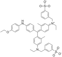
The Bradford assay uses a dye called Coomassie Brilliant Blue G-250. This dye contains multiple, negatively charged groups which bind tightly to positively charged amino acids, while the aromatic groups in the dye's core stack with aromatic residues. The dye binds arginine, tryptophan, tyrosine, histidine, and phenylalanine residues on the protein's surface, but binds arginine eight times more tightly than the others. This results in a coloration that is more arginine-dependent than protein dependent, as proteins with more surface arginines will give a higher absorbance than proteins at the same concentration with fewer exposed Arg residues.

The assay measures protein concentration due to the change in coloration of the dye upon complexing with protein. Free Coomassie dye has a max absorbance at ~460 nm, while the protein-complexed dye has a max absorbance at 595 nm. This shift allows detection of the amount of complexed dye, and therefore the total protein. However, the linearity of this assay breaks down at high protein concentrations due in part to the partial absorbance at 595 nm of the uncomplexed Coomassie dye.

Watch the Bradford assay walkthrough to see the specific steps involved in this experiment.