When entering your data and completing this week's calculations in Excel, be aware that you will be submitting your Excel spreadsheet this week. You should organize your spreadsheet with clear labels and headings. Points will be deducted if your spreadsheet is disorganized and it is difficult to find the required information. See the Assignment 4 instructions for details.

1. Calculate all initial reaction rates for all of your data in Part C using an Excel spreadsheet. You should plot your data to see how linear it is and to determine if any points need to be excluded by visual inspection. Remember that the initial rate condition, where rate equals the slope of a line, is only true very early in the reaction when [S] ≈ [S]_o. Later in your time course plot, we expect the initial slope to get smaller and smaller as [S] decreases. For this reason, you are justified in dropping later time points for the fastest reactions. In some cases, you may only be able to use the first 30 or 40 seconds. Monitor the y-intercept and the quality of trendline fit as you are judging how many later time points to drop.

Once you have decided how many data points to use for each condition, use the SLOPE function (SLOPE(y_values,x_values)) as in Lab 2 to determine slopes (ΔA₄₀₀/Δsec) from your data.

2. Convert your slopes to total assay activity in Catecholase Units (CU):

3. Convert CU to relative activity (defined as CU/μL of enzyme):

4. If you started your reactions by adding undiluted enzyme solution, skip to step 5. Otherwise, if you had to dilute your enzyme stock solution because it was too active, you will need to calculate undiluted Relative Activity the following equation.

5. Your Relative Activity measurements will be v_o for further analysis. Use Excel to create a calculated column of v_o divided by catechol concentration in the assay (v_o/[S]). Make an Eadie-Hofstee plot (as shown in Figure 2 of the Background) with v_o/[S] on the x-axis and v_o on the y-axis. Plot a linear trendline through your data, include the equation and R².

6. You could use the SLOPE and INTERCEPT functions to extract you kinetics parameters from your Eadie-Hofstee plot data. However, it is essential for a scientist to include an uncertainty estimate for any measured value. These Excel functions do not have statistical output. Therefore, we will use the more advance LINEST function to generate an array with advanced statistical output to calculate the slope and y-intercept parameters with their respective uncertainty values from your trendline.

In an Excel cell, enter = LINEST(y-axis_data, x-axis_data,,1)

For " y-axis_data" simply highlight your v_o cells with your mouse then press comma. Next highlight the relevant " x-axis_data" cells (the v_o/[S] data) with your mouse, press comma twice, then type "1)". After you press enter, you will see a value that should be identical to slope displayed on your plot. Once you press Enter, Excel will display the slope. To get the full analysis, you need to follow this procedure shown below:

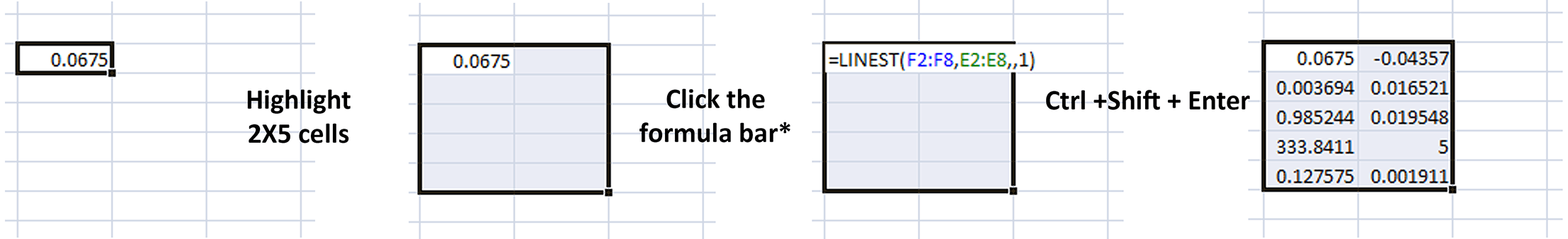
* The keyboard shortcut that is equivalent to clicking the formula bar is F2 on Windows or CTRL+U on Mac OS.

This returns the trendline parameters with advanced statistics. To understand everything in this array, read the help file for LINEST. The values of the array are briefly explained below:

You will only need the information from first two rows. The first row contains the slope and y-intercept (these should match the formula on your plot). The second row contains the standard errors for the parameters above given by the line fitting procedure. When you report your K_m and V_max, report these standard errors as your uncertainty. The uncertainty for your V_max/K_m estimate will be calculated as the square root of the sum of the squares of the relative uncertainties as explained in the Writing Guidelines.

7. Report these values on the spreadsheet for your lab section (links on Main Page).