Analyzing a Standard Curve Using Excel
In the example from the background section, I plotted the standard curve on graph paper and used visual graphical analysis to find the concentration of the unknown. However, it is far more accurate to use trendline analysis to derive a linear equation that relates absorbance to amount of protein.
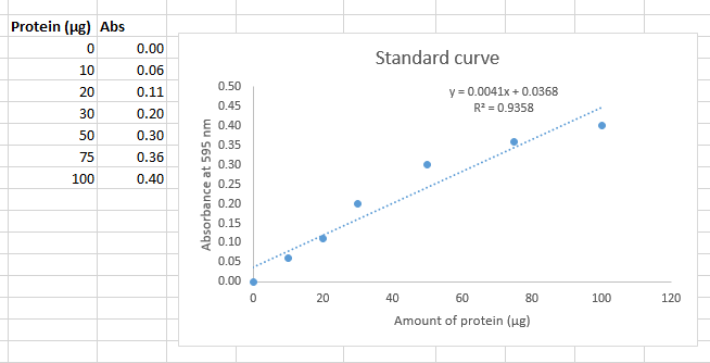
Using Excel, generate a scatter plot of corrected μg of BSA protein (x-axis) against absorbance (y-axis for your Bradford assay data as described above. For your standards, you recorded microliters of BSA added to each tube. Make sure that you convert to micrograms of BSA from each standard assay before plotting the data (the BSA solution was 1.0 μg/μl).
After generating a scatter plot in Excel with μg protein on the x-axis and corrected absorbance on the y-axis, select a data point, then right-click and choose Add Trendline from the dropdown menu. Select Linear as the trend type. To approximate the trendline parameters, go to the Trendline Options and check the boxes labeled Display Equation on Chart and Display R-squared Value on Chart, located near the bottom. The slope is the coefficient in front of x in the displayed equation. The R² value is the coefficient of determination, which indicates how well the data points fit the linear trendline. Although it is convenient to display these details on your plots during data analysis, when you present your plots in the Results section of your report, the title, legend, equation, and R² should appear in the figure caption rather than on the figure itself (see the Writing Guidelines for figure formatting requirements).
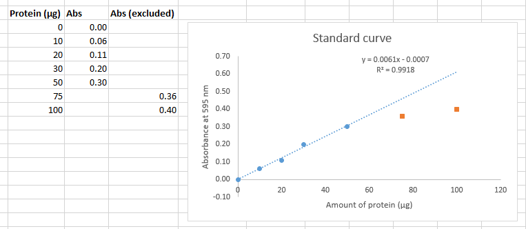
To exclude nonlinear data, you should move the y-axis points to a separate column then re-plot the graph and only fit the trendline to the linear data.
|
Deciding which points to omit, if any, is somewhat subjective. From the perspective of scientific ethics, it is essential that you openly declare in your writing which data you have omitted and provide your reasoning. Here are some simple rules you may apply in this course:
|
|
If you are planning on printing in black and white, make sure that the excluded data points are a different shape than the included dataset. To do this, select the excluded points on your plot, select "Format data series" from the Right-click menu (or from the menus select Chart Tools, Format, Format Selection). From the "Fill and Line" menu (Paint bucket icon), select "Marker" then expand "Marker Options" then select "Built-in" then choose the shape for your data points. |
As you can see, now the trendline more accurately describes the data (as demonstrated by the improved R2 value). However, we are still limited by the trendline, any measured absorbance above 0.300 for an unknown cannot be used to calculate the amount of protein. You must repeat the experiment by adding a smaller volume of sample so that you get values in range of the standard curve. Beer's Law is expected to break-down at some high concentration for each colorimetric assay in this experiment. You are therefore justified in dropping standard curve data at higher concentrations that deviate from linearity.
Generate the trendline parameters
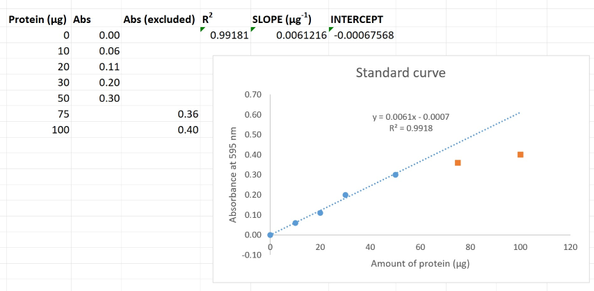
You should never use the equation given by Excel on the graph to convert absorbance to amount of protein. It often contains too few significant digits. Previously, you have used the SLOPE and INTERCEPT functions to get the parameters for the equation
$$ Absorbance = SLOPE \times \textit{Amount of Protein} + INTERCEPT \tag{1} $$The following is the syntax for the SLOPE, INTERCEPT, RSQ functions:
= SLOPE(y-values,x-values)
= INTERCEPT(y-values,x-values)
= RSQ(y-values,x-values)
For the y-values, simply highlight your y-axis cells (Absorbance) with your mouse then press comma. Next highlight the relevant x-values (Protein μg) cells with your mouse, type a closed parenthesis, and press Enter.
Rearranging Equation 1 gives
$$ \textit{Amount of Protein} = \frac{Absorbance - INTERCEPT}{SLOPE} \tag{2} $$Plug the SLOPE and INTERCEPT from the Excel functions into Equation 2
$$ P = \frac{A + 0.000676}{0.00612 \ \mathrm{μg}^{–1}} \tag{3} $$to get the equation to convert absorbance (A) to amount of protein in μg (P) for all your mushroom extract and reference protein samples for that assay. Clearly label these results in your spreadsheet.
Calculation of Protein Concentration
Calculate the amount of protein (in μg) for each sample of your mushroom extract and reference protein for the Bradford assay.
Next, divide the μg of protein you calculated by the volume (in μl) of sample you put into the tube before adding the colorimetric reagent.
Finally, calculate the average and standard deviation of these concentrations. You may discard any extreme outliers, particularly if you believe that you made a mistake.
Sample A absorbance __________ converts to __________ μg ÷ __________ μl = __________ μg/μl
Sample B absorbance __________ converts to __________ μg ÷ __________ μl = __________ μg/μl
Sample C absorbance __________ converts to __________ μg ÷ __________ μl = __________ μg/μl
Average __________ ± __________ μg/μl
Repeat these steps for the Lowry assay and for the BCA assay.
Finally, calculate the protein concentration from your direct UV measurement(s) using Beer's Law. The extinction coefficient and molecular weight of the most abundant isozyme are 99,030 M-1cm-1 and 63.9 kDa respectively. The absorbance units from the nanodrop, are scaled to a cm pathlength. No correction for the shorter pathlength is necessary. Make sure that you convert molarity (mol·L-1) to μg/μL units so that you can compare this measurement to the other assays. Once again, report the average and standard deviation.
For UV analysis of the papain sample, convert to concentration by multiplying absorbance by 0.4852 μg/μL . This number takes the extinction coefficient and molar mass into account.
Note: The unit Da or dalton is equivalent to u (atomic mass unit). Biologists tend to use Da to report the mass of macromolecules and chemists/physicists tend to use u for smaller molecules. If you haven't worked with atomic mass units in a while, for the purposes of calculations with fewer than four significant digits, 1.000 kDa = 1000 g/mol.