-
The National Institute of Standards and Technology in
Washington D.C., formerly called the National Bureau of Standards (NBS),
is responsible for maintaining accurate measures and weights in the U.S.
The NBS-10 Dataset consists of 100 weighings of a 10 gram prototype weight by NBS.
This 10 gram prototype weight was obtained by NBS in 1940.
It has been weighed once a week since then as a quality check on its weighing equipment and procedures.
The following article discusses the problem of investigating unknown measurement error with prototype weights:
Find the outliers using the boxplot.
Delete the outliers (see Part F of the SPSS Tutorial).
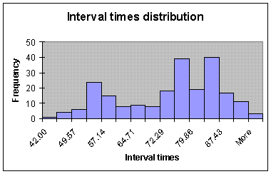
Construct a histogram of the NBS-10 dataset with a superimposed normal curve.
-
The center is the location of its axis of symmetry.
The spread is the distance between the center and one of its inflection points.
-
Heights of living things, weights of living things, lengths of inert
appendages (hair, claws, nails, teeth) of biological specimens in
the direction of growth, blood pressure of adult humans of fixed gender,
velocities of molecules in an ideal gas, measurement errors, IQ scores,
SAT scores.
