Describing Data
Now that we've covered the different types of measures that can be employed, we can explore some of the tools used to described the observations we've made.
I Describing Data
Once we have our measurements, we often want to get a sense of what these measurements (data) mean: In other words, we want to be able to describe what we have observed. One of the best ways to take a look at the scores we obtained is to create a distribution of scores.
For purposes of demonstration, let's assume that we have measured a group of students in terms of their age and their religious affiliation.
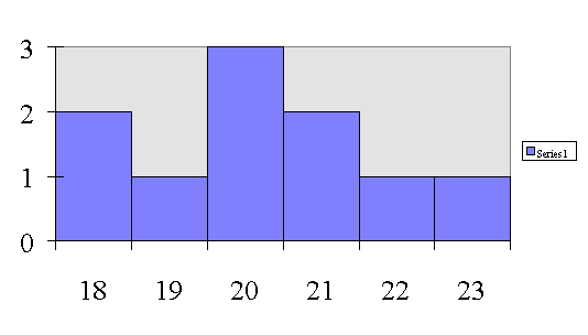
For Age we get the following scores:
18, 20, 21, 22, 19, 20, 20, 23, 18, 21
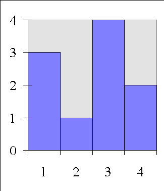
For Religious Affiliation we get the following scores:
(1 = Protestant, 2 = Buddhist, 3= Catholic, 4= Jewish)
1, 1, 3, 2, 4, 3, 3, 4, 1, 3
To explore the data we've collected, lets look at the distribution of these measurements.
A Distribution of scores simply means placing the scores we obtained in order (from smallest to largest).
Distribution of Scores for Age
18, 18, 19, 20, 20, 20, 21, 21, 22, 23
Distribution of Scores for Religious Affiliation
1, 1, 1, 2, 3, 3, 3, 3, 4, 4
Another useful way to look at the data is to put the data into what is called a Frequency Distribution. A frequency distribution simply means presenting the scores by noting how many times each score occurred.
Typically the way we show frequency distributions is to graph them on a plot, where the X - axis represents the scores, and the Y - axis represents how often each score occurred.
Frequency Distribution for AGE

Frequency Distribution for Religious Affiliation
So, one way that we can gain information
about our scores is to take a look at the distribution of the
scores.
What should you look for when examining distributions?
Several things to take notice of when looking at Distributions
1. Spread
How close the scores or data points are
How far apart the scores or data points are
2. Shapes
How the scores cluster together.
Common types of shapes and spreads (Bell-Shaped [normal curve], Peaked distributions, Flat distributions, Positive Skewed distributions, Negative Skew distributions)
However, there are also some descriptive statistics that we can calculate that will help us understand what our data look like.
Descriptive statistics simply describe what the scores obtained look like.
One very important descriptive statistic refers to the idea trying to identify what our most central score looks like. The most common score.
B Measures of Central Tendency
Score that best represents what is common.
These descriptive statistics are called measures of central tendency.
There are three measures of central tendency
1. Mode most frequently occurring score. (It is possible to have more than one mode or no mode at all).
Simply the score or scores that occur the most often
1, 1, 3, 4, 5, 8, 10
Mode is 1
1, 2, 3, 3, 3, 7, 8, 9, 9, 9
This distribution is bimodal (3 and 9)
2 Median The middle score. Score that cuts distribution in half.
Simply find the score that falls right in the middle of the entire distribution. If there is not a single point, then take the average of the two most middle scores.
1, 2, 5, 7, 9
The middle most score in this distribution is 5.
1, 2, 5, 7, 9, 10
The middle most score is the average of 5 and 7 (or 6).
3. Mean or mathematical average
Summary of Central Tendency:
All of these measures try to identify the most common or central score within a distribution.
Why three indexes?
When should each measure be used?
Take into account type of measured used:
| Mode | Median | Mean | |
| nominal | Yes | ||
| ordinal | Yes | Yes | |
| interval/ratio | Yes | Yes | Yes |
Should look at distributions as well.
Sometimes the Mode represents the central most score.
For example:
If you look at the distribution of how many years after marriage people get divorced you notice that there are two modes. So, in this case you would say that people are most likely to get divorced after 5 or 25 years of marriage.
However, if you had reported the mean or
median, say 15 years of marriage you would not have been as
accurate. Almost no one gets divorced at the 15 year point. 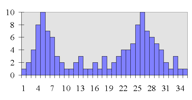
So, if distribution has several modes, probably best to report modes as the central most score.
However, sometimes the Median represents the central most score.
For example:
If you look at the distribution of how much
money attorney's make, you'll notice that a small group of
attorney make an enormous amount of money. These extreme scores
influence what the Mean score is -- because the scores are
averaged when calculating the mean. So, for instance, on average
attorney's might make 125 thousand dollars a year by looking at
the mean. However, the median score in this case more accurately
reflects the central most score. The median score is not
influenced by extreme scores in the same way that the mean is.
For example, the median score for attorney income might actually
be 55 thousand dollars. 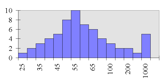
So, when extreme scores are present, the median is most likely to represent the central most score.
C Measures of Dispersion
Deals with how spread out the data is. These measure how far apart scores are from one another (how spread out is the data)
1. Range
Simply the distance from the highest to the lowest.
It is calculated by subtracting the lowest score from the highest score in the distribution.
2. Standard Deviation (SD)
Indicates, on average, of how far a set of scores are from the mean.
Indicates how spread out a set of scores are around the mean.
The smaller the SD, the more peaked or closer the scores are together.
The larger the SD, the more flat or spread out the scores are.
Importance of central tendency and dispersion.
This information is very useful for purposes of comparison with other scores.
If we describe any individual's score on a variable not in terms of their raw score, but in terms of means and standard deviations, can get a good idea of where that person lies, even with regard to other people within the distribution, or across different distributions.
For example. Say someone scores 45 on a math test and 75 on a biology test. Which one did they do better on in comparison to their classmates?
Some might say math, some might say biology, perhaps depending on what the mean of each test was ...... However, does knowing the mean really indicate how the person did in comparison to the rest of the class?
What if I tell you the mean on the biology test was 40, the mean on the math test was 70.... Well, we still don't quite know.....
but if I tell you the SD on the math test was 1.5, and the SD on the biology test was 12... then you know...
That is, the person scored over 3 standard deviations above the mean on the math test and less than one standard deviation above the mean on the biology test. In other words, the person was among the top scores on the math test – and came out right in the middle of the class on the biology test (remember 68-95-99 percent rule).
There is a very precise way to calculate how far any given score is above or below the mean in terms of standard deviations.
This score is called a z-score. A z-score is simply a way of describing any given score in a distribution in terms of its placement to the mean.
Z-scores are useful, because they tell you exactly where a score falls within a distribution, based upon the 68-95-99 percent rule.
Side note: You should always calculate a z-score when you get an exam, cause then you'll know precisely how you did in comparison to your classmates.
It is very easy to calculate a z-score.
Simply take the score in question, subtract the mean of the distribution and then divide by the standard deviation of the distribution.

Where,
![]() = mean or average of the distribution
= mean or average of the distribution
s = the standard deviation of the distribution.
So, if your z score is +2 you know you did very well on the exam.
However, if your z score is -2, then you know you didn't do so hot.
In short, z-scores are useful because they tell you where any given score falls within a distribution.