Ans: proj1-smithx.doc, where you replace Smith by your last name.
Ans: The two inner fences are located at Q1 - 1.5 x IQR and Q3 + 1.5 x IQR. The two outer fences are located at Q1 - 3.0 x IQR and Q3 + 3.0 x IQR. Extreme outliers are located to the outside of the outer fences. Mild or medium outliers are located between the inner and outer fences.
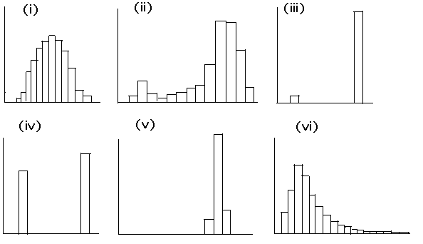
- The gender of all persons in a college class (male = 0, female = 1).
Ans: iv.
- The handedness of all persons in a college class (left handed = 0,
right handed = 1). Ans: iii.
- The heights of all married persons counted separately. Ans: i.
- The heights of all persons in families where both parents are
28 years old or less. Ans: ii
- The heights of all automobiles. Ans: v.
- The incomes of all persons in the U.S. Ans: vi.
Caution: what does it mean for histograms (b) and (c) to have bins of different widths?
| (a) |
|
(b) |
|
(c) |
|
Answers for Problems 5 and 6.
Answers for Problem 7.
- the incomes of all persons in the U. S.
Ans: A skewed histogram with a peak at about 35 or 40 thousand, but with a long right tail that extends all the way past 1 billion.
- the GPAs of all students at DePaul.
Ans: A bell-shaped histogram with peak around 3.0. There may be a secondary peak around 2.0, representing those students that have just come off of academic probation. The height of the histogram can only be nonzero in the range from 0 to 4.
- the number of years of schooling of all persons in the U. S.
Ans: A bell-shaped peak around 12 years (most people finish highschool, less people attend college).
- the IQs of all persons in the U.S.
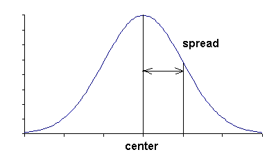
Ans: A bell-shaped curve with center at 100 and spread 15.
Ans: Statistical Package for the Social Sciences
- Create a new dataset.
Ans: Select New >> Data. Then type the data into the Data View.
- Change a variable name.
Ans: Change the variable name in the Name columns of the Variable View.
- Add a label to a variable.
Ans: Enter the label in the Label column in the Variable View.
- Import a dataset from an Excel file.
Ans: Select Import >> Data. Set the filetype to .xls and open the desired Excel file. Then indicate the worksheet you want to use and whether the variable names are in the first row.
- Print a dataset.
Ans: Select Analyze >> Reports >> Case Summaries. Select the variables that you want to print.
- Obtain Q0, Q1, Q2, Q3, and Q4 for a dataset.
Ans: Select Analyze >> Descriptive Statistics >> Explore... Click the Statistics button and check the Percentiles button.
- Obtain a histogram and a boxplot.
Ans: In addition to the answer 17f click the Plots button and select Histogram. The Stemplot is not needed.