TUTORIAL: t-tests in R.-

The following is a tutorial how to conduct a one-sample, two-sample, or paired-sample t-test in R created for my students and others that might find it useful. The t-test is one of the most basic methods of statistical analysis for continuous data. It is used to test for differences between a sample and population mean, or between the means of two samples.

Before beginning, you should have R, RStudio, and ggplot2, downloaded and ready for use. See my Beginning Work in R Tutorial.

Note that the code is included in the gray boxes below to make it easy to cut and paste. The explanations are interspersed in regular html.

To begin, you will need to set the working directory, open the file, and attach the variables. To set the working directory, use the setwd function. Select the location on your computer where you created a folder for the data and output files. R will look for your data file and save output files in this folder. I created a folder specifically for this t-test tutorial in my R_work folder.

You can check that the working directory was set correctly by using the "getwd()" command.

R should list the correct working directory as output once you hit enter.

Then we will open our data file. Data files can be generated in Excel by saving spread sheets as tab delimited text files. My example data file is called "data_RS_SL_HL.txt". It includes standard length (SL) and head length (HL) data for 50 male and 50 female anadromous (sea-run) threespine sticleback collected in Rabbit Slough, Alaska. The data are from a study published by Aguirre and Akinpelu (2010) on sexual dimorphism of head length in threespine stickleback that includes many Alaskan stickleback populations (click here for the pdf). We will use the SL data from just one anadromous population in this tutorial for simplicity. The data file is located on Github if you want to download it and use it in this tutorial (click here to download the data file). This data file has headers (variable names).

If you are using your own data file, make sure to indicate whether it has headers and attach the variable names to the data file and list the data.

Use the following commands substituting the name of your data file if necessary:

The first command "read.table("data_RS_SL_HL.txt", header=T)", should result in a listing of your data. The second command, "data=read.table("data_RS_SL_HL.txt", header=T)", assigns the name "data" to the data table and indicates that it has a header (T is for true indicating that the first row lists the variable names). The third command "attach(data)" attaches the variable names to the data file, and the final command "names(data)" lists the variable names. You should see "Sex" "Spec" "SL" "HL" as output for the variable names if you are using my example data file.

Now that we have our data ready, lets talk about t-tests. The t-test allows us to test for differences between a sample mean and the parametric mean of a population, or between the mean of two samples. It is based on a distribution called the t distribution worked out by W.S. Gosset published under the pseudonym "Student" while working at Guiness. The t distribution is important because it is appropriate for testing hypotheses based on sample data, which is the most common situation in applied statistics. The t distribution is also used to establish confidence intervals for sample means.

There are actually three types of t-tests that are commonly used in biology:

• The one-sample t-test
• The two-sample t-test
• The paired-sample t-test

Let's look at each in turn.

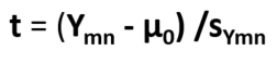
The one-sample t-test: The one-sample t test is the simplest statistical test involving continuous data and addresses the question: Is the sample mean from the data you have collected equal to that of the hypothesized population mean? That is, does your sample data come from the population of interest or not? It is applied when you only have data from one sample.

Because of the uncertainty related to sampling, two means will always differ even if they are samples of the same population. So how can we tell if the difference between our sample mean and the known parametric mean is biologically significant or simply due to sampling error? This is where the t-test comes in.

To conduct this test, you should have have a known parametric mean for the population of interest. This parametric mean is typically taken from the literature or given to you, and will be compared against the mean computed from the sample data that you collected. The null hypothesis that you are testing is that the sample mean is equal to the parametric mean. The alternative hypothesis is that the sample and parametric means differ. The equation is:

Where Y_mn is your sample mean, u₀ is the parametric mean of the sample, and S_Ymn is the standard error of your sample mean calculated as the sample standard deviation divided by the square root of the number of specimens in the sample.

This calculated t value is compared to the critical t value with n - 1 degrees of freedom, where n is the sample size. The degrees of freedom are a measure of the dimensions of independent variation and every statistical test has a standard equation for calculating the degrees of freedom. The critical t value is typically looked up in a table when conducting the test on pencil and paper. If the absolute value of the calculated t value is less than the critical value, the probability of getting the result if the null hypothesis is true is less than 0.05 or 5% (P < 0.05), so we reject the null hypothesis and conclude that our sample mean differs significantly from the parametric mean. Otherwise, we fail to reject the null hypothesis and conclude that there is no evidence that the sample and parametric means differ (the difference is not statistically significant). It is worth noting that if conducting the test on a computer, the probability of getting the calculated t value under the null hypothesis is computed directly.

Now, let's look at an example. Aguirre et al. (2008) computed the mean standard length (SL) of male and female anadromous threespine stickleback in Rabbit Slough as 66.71 mm based on three years of data. Does the mean SL calculated from a sample of 50 male and 50 female Rabbit Slough threespine stickleback measured in one year differ from this "parametric" population mean?

We will use the data available in the data_RS_SL_HL.txt file, which is from from Aguirre and Akinpelu (2010). Let's begin by computing the sample mean using the following script:

This gives us a sample mean of 65.18 mm SL compared to the population mean of 66.71. The means obviously have different values but this will always be the case when dealing with samples because of inevitable sampling error. We want to know if this difference is statistically significant. We will use a one-sample t-test to answer this question. Input the following script:

This script tells R to conduct a t-test using the SL variable in your open data file. mu=66.71 gives the value of the parametric mean against which the sample mean will be compared. This gives us the following output:

One Sample t-test

data: data$SL
t = -4.8736, df = 99, p-value = 4.172e-06
alternative hypothesis: true mean is not equal to 66.71
95 percent confidence interval:
64.55131 65.80049
sample estimates:
mean of x
65.1759

As you can see, the calculated t value is quite extreme at -4.8736. Remember that our sample consists of 100 specimens (50 males and 50 females) so the degrees of freedom are 100 - 1 = 99. The probability of getting a difference of this magnitude if the null hypothesis is true is 4.172e-06, which is quite small and much less than 0.05, so we reject the null hypothesis and conclude that the sample and parametric means differ significantly. Our conclusion can be written as:

The mean SL of the sample of Rabbit Slough stickleback measured differs significantly from the known mean of the population (one-sample t-test, t = -4.8736, df = 99, p < 0.001).

Note that the output also lists the sample mean (65.1759) and the 95% confidence interval of the sample mean, 64.55 - 65.80, which does not overlap with the parametric mean.

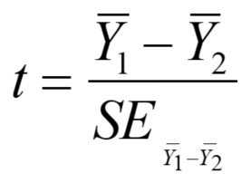
The two-sample t-test: The two-sample t-test is probably what most people think of when they hear t-test. It is used to test whether the means of two samples differ, when the individuals within each sample are independent of each other. That is, you have a random set of individuals measured in sample 1 and another random set of individuals measured in sample 2, and you want to test whether the means of those two samples differ significantly.

The equation for the two-sample t-test is very similar to that of the one-sample t-test (Whitlock and Schluter, 2015):

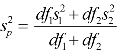
The main differences are that you have two sample means in the numerator instead of one sample mean and a parametric mean, and the denominator is a standard error of the difference between sample means instead of a simple standard error of the mean of one sample. To compute the standard error of the difference between means, you first need to compute the pooled sample variance using the following equation:

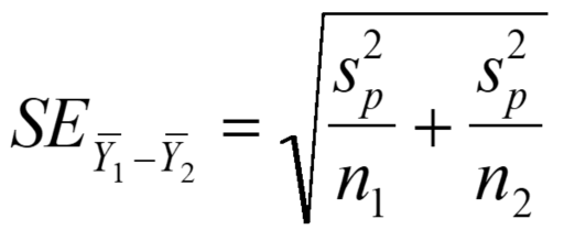
Where df₁ and df₂ are the degrees of freedom of samples 1 and 2, respectively (calculated as the number of individuals in each sample - 1, so n₁ - 1 and n₂ - 1), and s₁² and s₂² are the variances for sample 1 and 2, respectively.

You then calculate the standard error of the difference between sample means using the following equation:

Where s²_p is the pooled sample variance calculated above, and n₁ and n₂ are the number of individuals in samples 1 and 2, respectively.

This gives us our test statistic, the t value. As with the one-sample t-test, if the probability of getting our observed t value under the null hypothesis (the sample means do not differ significantly) is less than 0.05 or 5%, we reject the null hypothesis and conclude that our sample means differ significantly.

Let's go back to our Rabbit Slough stickleback data. Does standard length (SL) differ significantly between male and female threespine stickleback in Rabbit Slough? Our data file should already be open and ready to use, if not, see the section above on how to do this in the one-sample t-test. The t-test assumes that sample variances are homogeneous, so before we conduct the actual t-test, we should test this assumption. There are a number of tests of homogeneity of variances. We will use Bartlett's test, which is one of the best known. Input the following code:

This code is telling R to use Bartlett's test to test whether the variance in standard length ("SL") is homogeneous between the groups designated by our "Sex" variable (males and females).

The output we get is:

Bartlett test of homogeneity of variances

data: SL by Sex
Bartlett's K-squared = 3.1063, df = 1, p-value = 0.07799

Which indicates that the variance in SL does not differ significantly between males and females because P>0.05, although it is close!

Now we can conduct the two-sample t-test by inputing the following code:

Which tells R to conduct the two-sample t-test with SL as the variable being tested and Sex indicating the groups. By default, R assumes that the variances are not homogeneous and conducts a variant of a t-test, Welch's two-sample t-test, that can handle violations of this assumption. In our case, the variances were homogeneous so we can conduct a standard two-sample t-test by specifying this using the "var.equal=TRUE" command.

The output we get is:

Two Sample t-test

data: SL by Sex
t = 8.2954, df = 98, p-value = 5.92e-13
alternative hypothesis: true difference in means is not equal to 0
95 percent confidence interval:
3.060745 4.985655
sample estimates:
mean in group F mean in group M
67.1875 63.1643

Remember that we have 50 males and 50 females, so the degrees of freedom for the test are (50-1) + (50-1) = 98. Our t-value is quite extreme such that the probability of getting a t-value of this magnitude if the null hypothesis is true is 5.92e-13, which is way below 0.05. So we reject the null hypothesis and conclude that SL differs significantly between male and female threespine stickleback from Rabbit Slough (two-sample t-test, t = 8.2954, df = 98, p < 0.001).

Note that our output also gives us 95% confidence intervals for the difference between means (3.060745 - 4.985655) and the mean SL for our test groups, females (67.1875) and males (63.1643). Females are substantially larger than males in this population, as is typically the case in threespine stickleback.

The paired-sample t-test: Coming soon.

SUGGESTED READING:

For a general treatment of statistical tests and t-tests, see:

-Whitlock, M., and D. Schluter. 2015. The analysis of biological data. Roberts and Company Publishers. Greenwood Village.

For an R focused treatment of these topics, see:

-Crawley, M.J. 2015. Statistics, an introduction using R. John Wiley & Sons. West Sussex.

OTHER REFERENCES CITED:

-Aguirre, W.E., and O. Akinpelu. 2010. Sexual dimorphism of head morphology in threespine stickleback. Journal of Fish Biology 77:802-821.

-Aguirre, W.E., K.E. Ellis, M. Kusenda, and M.A. Bell. 2008. Phenotypic variation and sexual dimorphism in anadromous threespine stickleback: implications for postglacial adaptive radiation. Biological Journal of the Linnean Society 95:465-478.