TUTORIAL: BOX PLOTS IN R.-

The following is a tutorial for creating box plots in R for my students and others that might find it useful. It is also a learning tool for me since I am relatively new to R.

Box plots are a popular type of graph for comparing a continuous variable (typically plotted on the Y axis) between several groups (a categorical variable plotted on the X axis). See below for visual depictions. The box includes the 50% middle portion of the data with a horizontal bar in the box representing the median. The bars spanning up and down from the 50% box represent the non-outlier range (first and fourth quartiles). Outliers, if present, are depicted as isolated points beyond the range bars.

Before beginning, you should have R, RStudio, and ggplot2, downloaded and ready for use. See my Beginning Work in R Tutorial.

Note that the code is included in the gray boxes below to make it easy to cut and paste. The explanations are interspersed in regular html.

To begin, you will need to set the working directory, open the file, and attach the variables. To set the working directory, use the setwd function. Select the location on your computer where you created a folder for the data and output files. The location I use is listed below. R will look for your data file and save output files in this folder.

Then open your data file. Data files are often generated in Excel by saving spread sheets as tab delimited text files. My data file is called "data.txt". You should give your data a name and indicate whether it has headers (variable names). Then attach the variable names to the data file and list the data.

Use the following commands substituting the name of your data file if necessary:

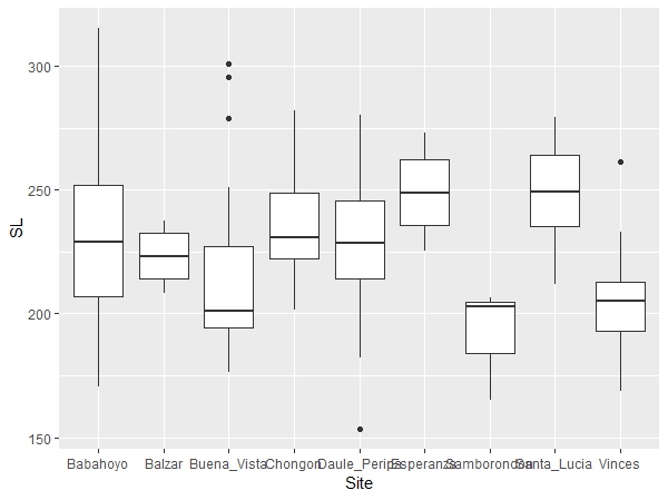
The example data file includes standard length (SL) data for a Neotropical fish species, Brycon alburnus, collected in river and artificial impoundment sites in western Ecuador. We will use these data to make a simple box plot figure using the following command:

"ggplot" is calling the ggplot2 program to create a plot and it will use your "data" file. "aes" is short for aesthetic and is defining your x and y variables in this case. SL will appear on the Y axis and Site on the X axis. The "aes" function has other uses too. "geom_boxplot()" is specifying the plot type as a box plot. The plot will appear in the bottom right window of RStudio under the Plot tab. You can easily save this plot as an image or pdf and indicate the image size using the export function in RStudio.

To eliminate gray background and grid lines use "theme_classic()":

To color the box plots by type, use the "fill" command. In this case, type refers to whether the fish were collected from artificial lake (formed after dam construction) or river sites.

You can also use the fill function to make subgroups within groups. Because there are different sexes within each X site, using the following command creates different box plots by sex within sites.

Note that sex could not be determined for the last few sites so it is simply labeled as "U" for unidentified sex. Some fish were also tentatively identified as male but there was some uncertainty with this identification so they are labeled as "M?". For the sites for which males and females could be identified (e.g., Babahoyo, Chongon, Daule Peripa), females appear to be somewhat larger, which is relatively common in fishes.