
|
|
|
|
TUTORIAL: ANOVA in R.- The following is a tutorial on how to conduct a one-way ANOVA in R created for my students and others that might find it useful. ANOVA is one of the most powerful and commonly used methods of statistical analysis for continuous data. It is used to test for differences between two or more sample means and allows partitioning of variation into amonng and within group components. Before beginning, you should have R, RStudio, and ggplot2, downloaded and ready for use. See my Beginning Work in R Tutorial. Note that the code is included in the gray boxes below to make it easy to cut and paste. The explanations are interspersed in regular html. To begin, you will need to set the working directory, open the file, and attach the variables. To set the working directory, use the setwd function. Select the location on your computer where you created a folder for the data and output files. R will look for your data file and save output files in this folder. I created a folder specifically for this ANOVA tutorial in my R_work folder.
|
|
setwd("C:/1awinz/R_work/anova_tutorial") |
R should list the correct working directory as output once you hit enter. Then we will open our data file. Data files can be generated in Excel by saving spread sheets as tab delimited text files. My example data file is called "stickleback_SL_anova.txt". It includes standard length (SL) data for male and female threespine sticleback from five lake, stream, and anadromous Alaskan populations. The data are from a study published by Aguirre and Akinpelu (2010) on sexual dimorphism of head length in threespine stickleback (click here for the pdf). We will use the SL data from a few populations in this tutorial for simplicity. The data file is located on Github if you want to download it and use it in this tutorial (click here to download the data file). This data file has headers (variable names). If you are using your own data file, make sure to indicate whether it has headers and attach the variable names to the data file and list the data. Use the following commands substituting the name of your data file if necessary:
|
|
read.table("stickleback_SL_anova.txt", header=T) data=read.table("stickleback_SL_anova.txt", header=T) attach(data) names(data) |
The first command "read.table("stickleback_SL_anova.txt", header=T)", should result in a listing of your data. The second command, "data=read.table("stickleback_SL_anova.txt", header=T)", assigns the name "data" to the data table and indicates that it has a header (T is for true indicating that the first row lists the variable names). The third command "attach(data)" attaches the variable names to the data file, and the final command "names(data)" lists the variable names. You should see "Sex" "Spec" "SL" "HL" as output for the variable names if you are using my example data file. Now that we have our data ready, lets talk about the analysis of variance (ANOVA). ANOVA is one of the most commonly used and powerful statistical methods available. It allows us to test whether there are significant differences in means among multiple groups. There are multiple forms of ANOVA that allow one to test different types of experimental designs. The one-way ANOVA is the simplest form of this test and is used when there is one response variable and one categorical variable that divides subjects into groups. Typically ANOVA is employed when there are three or more groups. It can be employed when there are only two groups, however, the simpler two-sample t-test would be typically employed in this case. ANOVA works by partitioning the variance in the data into Among Groups (or groups) and Within Groups (or error) components. These estimate the variance in different ways such that the Among Groups estimate of variance will be inflated if there is an extra component of variation reflecting differences in the means among groups. The Within Groups estimate gives an estimate of variance that does not take this among groups component into account. As a result, the ratio of the Among Groups to Within Groups variance estimates will be approximately 1 if the means of the different groups are homogeneous but will be significantly greater than 1 if the group means differ. This ratio is called the F ratio and the F distribution is used to determine how large F has to be to conclude that there is a significant difference among groups. In terms of the calculations, a Groups Sum of Squares and an Error Sum of Squares are computed and divided by their respective degrees of freedom (K-1 for the groups and N-K for the error, where N is the total number of individuals in the study and K is the number of groups) to give the Mean Squares, which are estimates of the variance. The MSGroups and MSError are divided to give the F ratio, which is compared to the critical F ratio using an F table with K-1 and N-K degrees of freedom. ANOVA has the interesting property that the SSGroups and SSError add up to the total Sum of Squares computed using all the data and the grand mean. The Groups and Error degrees of freedom also add up to the Total degrees of freedom (N-1). The results of the ANOVA are then presented in a table format, which includes the P value, the probability of obtaining the calculated F statistic if the null hypothesis (which is tthat there are no significant differences among group means) is true. If P < 0.05 or 5%, one rejects the null hypothesis and concludes that there are significant differences among group means. Otherwise, one fails to reject the null hypothesis. If the ANOVA is significant, additional multiple comparisons tests are perfomed to determine which groups differ from each other. All groups may be significantly different from each other or it may just be one group that is different from all the rest. Lets work through an example. We will take data from a study by Aguirre and Akinpelu (2010), who examined sexual dimorphism in head length of several populations of Alaskan threespine stickleback. For this example, we will only use standard length (SL) data from five of the samples that they measured: three lake populations: Beaverhouse (BH), Mud, and Bear Paw (BP), a stream population: Little Meadow Creek (LMC), and an anadromous population: Rabbit Slough (RS). Sex was also identified for the specimens measured but we will not use those data. Does mean SL differ among these ecologically heterogeneous populations? We will conduct an ANOVA to answer this question. First, let's compute the mean standard length for each sample using the aggregate function. Type in the following command:
|
|
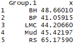
aggregate(SL, list(Pop), mean) |
This command is telling R to aggregate our specimens for the variable SL by the population (Pop) that they belong to, and list the mean SL for each population. You should get output like this: |
|
The table lists the mean SL for each of our five samples (BH, BP, LMC, Mud, and RS). It is clear that there is quite a bit of variation in mean SL, but are these differences statistically significant? A one way ANOVA can be conducted using this simple command in R:
|
|
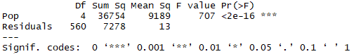
summary(a1<-aov(SL~Pop)) |
The "aov" command tells R to conduct an analysis of variance using SL as the response variable and Pop (population) as the categorical variable to split individuals into groups. The "a1<-" portion is telling R to save the analysis and name it a1. The "summary" command tells R to list the ANOVA table. Otherwise, R will just perform the ANOVA but not display output. The following output should appear: |
|
|
Note that our value for the F ratio (F value) is 707, which is huge! Remember that we expect an F value of about 1 if there is no significant among groups effect. The P value, listed as "Pr(>F)" is < 2-16, which is way below 0.05 so we can reject the null hypothesis and conclude that standard length differs significantly among the five Alaskan stickleback populations sampled (ANOVA, F = 707, df = 4, 560, P<0.001). So we know that there is a significant difference among sample means but how do we know which samples differ from which? This is where the multiple comparisons test comes in. We will use Tukey's Honestly Significant Difference test (Tukey HSD), which is one of the most commonly used. Input the following command in R:
|
|
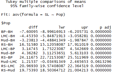
TukeyHSD(a1) |
You should get the following output: |
|
|
The Tukey HSD procedure conducts a series of pairwise comparisons between means, listing the difference between each pair of means, the 95% confidence intervals for the difference between means, and the P value for the pairwise test of the difference between means (p adj). It seems that all samples differ in SL from each other with the exception of Mud Lake and Little Meadow Creek! The Rabbit Slough sample is particularly large relative to the other samples, which makes sense since anadromous populations in Alaska are known to typically be larger in body size than resident freshwater populations. |
|
SUGGESTED READING: For a general treatment of statistical tests and ANOVA, see: -Whitlock, M., and D. Schluter. 2015. The analysis of biological data. Roberts and Company Publishers. Greenwood Village. For an R focused treatment of these topics, see: -Crawley, M.J. 2015. Statistics, an introduction using R. John Wiley & Sons. West Sussex.
OTHER REFERENCES CITED: -Aguirre, W.E., and O. Akinpelu. 2010. Sexual dimorphism of head morphology in threespine stickleback. Journal of Fish Biology 77:802-821.
|
Date last modified: Sep/6/19
Date created: Sep/6/19 (by: Windsor Aguirre)