Brief Overview of Sampling
Probability Theory
Working through an example:
Population: Eight students in this class.
Study Population & Sample Frame: Erin, Trina, Jean, Jose, Rich, Mark, Ruth, Rob
Interested in estimating how many beers these students drank on Thurs. night.
This is how many they actually drank:
| Erin | Trina | Jean | Jose | Rich | Mark | Ruth | Rob |
| 3 | 1 | 0 | 2 | 3 | 4 | 6 | 5 |
The mean or average for these eight students is: 3.0 (24/8=3)
Through sampling procedures, we want to estimate how many beers these students drink on a Thurs. night.
Let's say we take a sample of two people from this Sample Frame
Erin & Trina: (3+1)/2 = 2 beers (sample statistic or population parameter)
How accurate is this estimate?
Now let's say we take a sample of four people from this Sample Frame
Erin, Jean, Rich, & Ruth (3+0+3+6)/4 = 3 (sample statistic or population parameter)
As you can see, typically the larger the sample the more accurate the estimate.
How much confidence to place on each estimate?
Key Idea: Sampling Probability Theory lets us estimate how much confidence we can put into the parameters we can up with.
Sampling Theory is based on the probably (the odds) that the sample we chose is close to the population.
In order to understand Sampling Theory, lets work through the following example.
Let's take a look what we would get if we were to pull out all possible samples of two from this group.
So, let's say we pull out every possible combination:
Erin & Trina
Erin & Jean
….
Ruth & Rob
What we have is a total of 28 possible samples the size of two.
Next, lets calculate the mean (the average) of each of these samples.
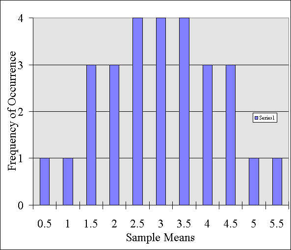
The means of all of these samples looks like the following:
If I were to graph these values on a chart it would look like this:

This graph, is called a distribution. I am simply listing each score or mean obtain and noting how often it occurred. This type of graph is called a sampling distribution because it represents a set of sample means.
By looking at this distribution, we can learn something about all of the different possible combinations of samples that it is possible to draw out.
For instance, how likely is it, if I sample two people that their mean score is going to be say 0.5? How likely is that going to happen? Based on this distribution, I know that it is not very likely to happen. In fact, it is only going to happen 1 out of 28 times. Or it has a 3.5% chance of happening (1/28).
In other words, the probability of pulling two people out with such a low mean has a very low probability of occurring.
On the other hand, how likely is it that the average of two people's scores are going to be between say 2 and 4? It is probably going to happen a lot. In fact, based on this distribution, we know it will happen 18 out of 28 times. That is, 64% percent of the time, a sample of any two people's scores will average out to be between 2 and 4.
Now, lets see what happens with when we sample four people at a time.
So, we have
Erin, Trina, Jean, Jose
….
Rich, Mark, Ruth, Rob
This time there are 70 possible combinations of samples the size of four.
If we were to calculate the mean score for each sample. We would have 70 sample means.
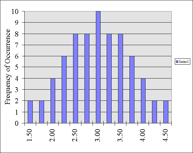
If I were to graph these 70 sample means they
would look like this:

By looking at this distribution, we can learn something about all of the different possible combinations of samples that it is possible to draw out.
For instance, how likely is it, if I sample four people that their mean score is going to be say 0.5?
This time around, it will be impossible to pull out four people that have an average score that is that low.
On the other hand, how likely is it that the average of four people's scores are going to be between say 2 and 4? It is probably going to happen a lot. In fact, based on this distribution, we know it will happen 62 out of 70 times. That is, 88% percent of the time, a sample of any four people's scores will average out to be between 2 and 4.
So, what happens as you increase sample size?
If we only took one sample of two people - we have a 64% chance of our sample being pretty close to 3 (between 2 and 4).
However, our odds get much better when we take a larger sample. That is, the chance of getting a good estimate (say between 2 and 4) is 88% if our sample size is larger (has four people).
When you look at these two distributions, what do you notice that is different about them?
How spread out the scores are.
If the distributions are peaked, then any given sample is more likely to be a pretty good estimate of our population.
If the distributions are rather flat, the any given sample is less likely to be a good estimate of our population.
There is a way to calculate how spread out the numbers are: This is typically called the Standard Deviation. That simply refers to on average, how far a set of scores are away from the mean score in the distribution.
In probability theory it is called the standard error or sampling error.
So, the larger the sampling error the less likely any given sample serves as a good estimate of the population.
Moreover, sampling distributions have special properties which make them very useful for estimating how accurate a parameter is.
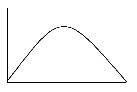
Sampling distributions are Normal Distributions. That means that they are symmetrical.

All normal distributions have very special properties. In particular,
the 68-95-99 rule applies.
68% of all scores fall within (plus or minus) one standard deviation of the mean.
95% of all scores fall within two standard deviations of the mean.
99% of all scores fall within three standard deviations of the mean.
For example:
Lets say that I know that the mean of the distribution above is 50.
Let's also say that I know that the standard deviation or sampling error is 5. That is, on average, the sample means are roughly 5 points from the middle score.
I now know that 68% of all of my scores are going to fall between 45 and 55.
Moreover, I know that 95% of all of my scores are going to fall between 40 and 60.
These examples illustrate how probably theory works, but in the real world, we can't take every possible combination of samples and build a distribution.
What happens is that we take a single sample, and work our way back.
That is, if I take a single sample. What do I know about that sample, based upon probably theory?
1. I know that there is a 68% chance that the sample falls within one standard deviation of the true value of the population.
2. I know that there is a 95% chance that the sample falls within two standard deviations of the true value of the population.
3. I know that there is a 99% chance that the sample falls within three standard deviations of the true value of the population.
So, we take a sample. Calculate a mean for that sample (statistic). We use this mean as the parameter or estimate of our population.
Based on upon sampling theory, we assume that we are 68% confidence that our parameter or estimate is within one standard deviation of the true population value. How confident we are that our sample actually falls near the true population value, is called a Confidence Level. This is simply how likely it is that our sample falls near the true population value.
Moreover, since we can estimate what the standard deviation or sampling error is, we can also calculate a Confidence Interval, which is simply an estimate of how far away we think our population parameter is from the actual population mean.
To calculate the confidence interval, we simply take our population parameter and add and subtract the sampling error.
For example.
Let's say I randomly ask 100 DePaul students how many beers they drank last night.
The mean (statistic) is 4.5
The parameter for our population is then 4.5
I also find out that the sampling error is 0.5
So, our confidence Interval is 4 to 5. ( 4.5-0.5 and 4.5+0.5) Simply going out one standard deviation each from from our parameter.
How certain of this are we? Our Confidence Level is 68%. (we only went out one standard deviation -- one sampling error).
However, we may want to be more accurate.
We can increase our confidence level by going out two standard deviations.
So, our confidence interval is then 3.5 to 5.5
Now we are 95% certain about this estimate.
If we want to be even more certain, we simply increase our Confidence interval.
So, we could be 99% certain of that DePaul students drank between 3 and 6 beers on average last night based upon asking 100 people.