To Lecture Notes

IT 223 -- 1/31/11

Review Questions

1. What is a bivariate normal dataset?

   Ans: A bivariate dataset that is univariate normal in any direction.

2. How many statistics are needed to parsimoniously describe a bivariate normal dataset?

   Ans: 5: x, y, SD_x, SD_y, and r.

3. How many statistics are needed to parsimoniously describe a multivariate normal dataset with m variables?

   Ans: m means + m sds + m(m-1)/2 pairwise correlations for a total of 2m + m(m-1)/2 = m²/2 + 3m/2 parameters.

4. Give a situation where there is perfect association causality between two variables x and y, but the correlation is close to 0.

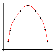
   Ans: A situation where the response curve is nonlinear as in the following image. The correlation is zero, but there is perfect causality.

   

5. If there is a linear association between x and y, what does the R-squared value tell you?

   Ans: It tells you the proportion of variation in the dependent variable that can be explained by x.

6. Compute the correlation r of this dataset "by hand" using SPSS (not using Analyze >> Correlate >> Bivariate).

   x	y
   1	1
   2	3
   3	2
   4	4

   Ans: x = 2.5, y = 2.5, SD_x+ = 1.290994, SD_y+ = 1.290994, Now compute z_x = (x-x)/SD_x+, z_y = (y-y)/SD_y+, and the products z_x z_y.

   Here is a table of the calculations:

   x	y	zx	zy	zx zy
   1	1	-1.161895	-1.161895	1.35
   2	3	-0.387298	0.087298	-0.15
   3	2	0.387298	-0.387298	-0.15
   4	4	1.161895	-1.161895	1.35

   The average of the products is (1.35 + (-0.15) + (-0.15) + 1.35) / 4 = 0.60. Multiply this by the correction factor n / (n-1) to obtain the correlation:

   r = n / (n-1) * 0.6 = 4 / 3 * 0.6 = 0.8.

7. In the Bears85 dataset, if the variables Meter and Kilo were not provided, how would you calculate them with Transform >> Compute Variable? There are 2.54 cm/in and 2.205 lb/kg.

More about Correlations

• See the Cautions Section in Linear Correlation

• The r-squared value r² measured the proportion of variation in the dependent variable that can be attributed to the independent variable.

• Correlation does not always imply causation.

• Correlation does not indicate the strength of a nonlinear relationship.

• Outliers can distort the correlation. They usually make it smaller.

Linear Regression

• The goal of linear regression is to find the line (or other curve) of best fit for a dataset.

• Names for the regression line:
  Regression Line (the best straight line equation for predicting y from x)

  Line of Averages (the line that connects the averages of the y-values in thin vertical rectangles)

  Least Squares Line (the line that minimizes the sum of the squares of the residuals)

  Linear Trend Line

• Linear Regression

Linear Regression Analysis with SPSS

1. Use SPSS to do the following with this dataset:

   x	y
   1	1
   2	3
   3	2
   4	4

   1. Create a scatterplot of y vs. x.

   2. Compute x, y, SD_x, and SD_y, and r. Use these statistics to compute the regression line.

   3. Verify your answer in 1b with SPSS.

2. Use SPSS to do the following using the Bears Dataset. Meter is the x-variable; kilo is the y-variable. See Part P of the SPSS Tutorial for help.
   1. Form a scatterplot of y vs. x.

   2. Compute x, y, SD_x+, and SD_y+, and r. Use these statistics to compute the regression line

   3. Find the regression parameters a and b. Use them to obtain the the regression line.

   4. Graph the residual plot of residuals (y-axis) vs. predicted values (x-axis).

   5. Interpret the residual plot.

   6. Graph the normal plot of the residuals.

   7. Interpret the normal plot of the residuals.

3. Collect data for the period of a pendulum (y-variable) vs. the length of the pendulum. Use the online stopwatch to time ten periods of the pendulum for each length. Then divide by 10 for one period. (One period is once forward and back for the pendulum.)

   Such data is included in the Pendulum Dataset. The time for 10 periods period is measured in seconds; the length is measured in centimeters. Transform the data to obtain x as the pendulum length in meters and y as the pendulum period in seconds.

   1. Plot the scatterplot of y vs. x.

   2. Compute the regression line.

   3. Locate the r-squared value on the regression plot. Verify that it is equal to r², where r is the correlation.

   4. Plot the residual and normal plots.

   5. Transform the x-variable by taking the square root of the length. Then repeat steps a, b, c, and d.

      Note: from physics, period = 2 π √length/g, where π = 3.14159265 and g = 9.80665 m/sec² is the acceleration of gravity.

Project 3

• Go over Project 3.