Graph lecture Notes

Introduction to Graph

Graphs

1. Basic definitions

Graph G = (V, E) where V is a set of vertices and E is a set of edges. Each edge e Î E is a 2-tuple of the form (v, w) where v, w Î V, and e is called an incident on v and w.
An edge may be directed or undirected.
An edge may also have a weight.
A path is a sequence of vertices connected by edges, and represented as a sequence in 2 ways:
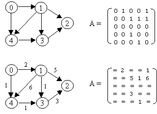
- (v₀, e₁, v₁, e₂, v₂,..,v_n-1, e_n, v_n) -- alternating vertices and edges
- (v₀, v₁, v₂,..,v_n-1, v_n) -- vertices only
A graph is connected if, for any vertices v and w, there is a path from v to w.

2. Graph Representations

Adjacency matrix
- n by n matrix, where n is number of vertices
- A(i,j) = 1 iff (i,j) is an edge, or 0 otherwise
- For weighted graph: A(i,j) = w (weight of edge), or positive infinity otherwise
Adjacency list
- Each vertex has a linked list of edges
- Edge stores destination and label
- Better when adjacency matrix is sparse
Incidence Matrix
- n by e matrix , where n is the number of vertices and e is the numbre of edges
- A(i,j) = 1 if and only if vertex i is an end point of edge e_j

3. Theorem :

If G is agraph with m edges and n vertices { v_i : i = 1,.. n} , then

S d(v_i) = 2 m .

Corollary: In any graph, there are an even number of vertices of odd degree.

4. Simple Graph :

A graph with no parallel edges or loops.

Some examples of simple graph

Complete graph with n vertices : K_n (there is an edge between every pair of vertices.
Bipartite graph : The set of vertices consists of two disjoint sets V₁ and V₂ and all the edges are of the form (v₁, v₂) with v₁ in V₁ and v₂ in V₂ .
Completer bipartite graph of m, n , K_m,n

5. Isomorphisms of Graphs

Graphs G₁ and G₂ are isomorphic if there is a one-to-one, onto function f from the vertices of G₁ to the vertices of G₂ and a one-to-one , onto function g from the edges of G₁ to the edges of G₂ , so that an edge e is incident on v and w in G₁ if and only if the edge g(e) is incident on f(v) and f(w) in G₂. The pair of functions f and g is called an isomorphism of G₁ onto G₂.

Theorem : Graphs G₁ and G₂ are isomorphic if and only if for some ordering of their vertices, their adjacency matrices are equal.

Corollary : For simple graphs G₁ and G₂, they are isomorphic if and only if there is a one-to-one, onto function f from the vertex set of G₁ to the vertex set of G₂ satisfying the following: Vertices v and w are adjacent in G₁ if and only if the vertices f(v) and f(w) are adjacent in G₂.

6. Planar Graph

A graph is planar if it can be drawn in the plane without its edges crossing.

Euler's Formula for Planar Graph

for any planar graph G, we have :
f = e - v + 2 where f = number of faces (contiguous region) ,
e = number of edges and v = number of vertices .

In any simple, connected, planar graph G , we always have e £ 3v - 6

K₅ and K_3,3 are not planar.

Kuratowski's Theorem : A graph G is planar if and only if G does not contain a subgraph homeomorphic to K₅ or K_3,3 .

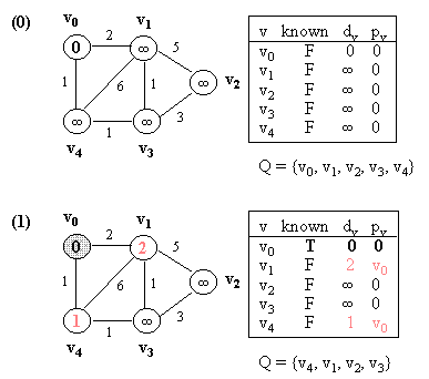
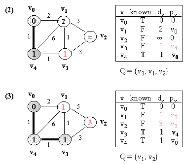
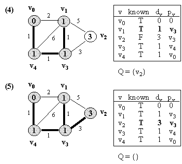
7. Dijkstra's Shortest-Path Algorithm

Input : A connected weighted graph with positive weighted, vertice a and z
Output : L(z) , the length of a shortest path from a to z .

1.  procedure dijkstra(w,a,z,L)
2.       L(a) := 0 
3.       for all vertices x ¹  a do 
4.           L(x) := ¥
5.         T := set of all vertices
6.      // T is the set of vertices whose shortest distance from a has 
7.      // not been found
8.      while  z  Î  T do 
9.           begin 
10.           choose v Î T with minimum L(v)
11.           T := T - {v}
12.           for each x Î T adjacent to v  do 
13.              L(x) := min{ L(x), L(v) + w(v,x)}
14.           end 
15.   end dijkstra

For input consisting of n-vertex, simple, connected, weighted graph,
Dijkstra's Algorithm has worst-case run time Q (n²) .

Euler Cycle (path)

A cycle (path) in a graph G that includes all of the edges (as a consequence, also includes all the vertices) is called an Euler cycle (path).

The necessary and sufficient condition for a graph G to have a Euler cycle is

G is connected and
every vertex in G has even degree

The necessary and sufficient condition for a graph G to have a Euler path is

G is connected and
every vertex except two in G has even degree

Hamiltonian Cycle

A cycle in a graph G that contains each vertex in G exactly once, except for the starting and ending vertex that appears twice.

A path in a graph G that contains each vertex in G exactly once is called a Hamiltonian path.

There is no well-known necessary and sufficient condition for the exitence of a hamitonian cycle in a given graph G.

More about Hamiltonian circuits

The Traveling saleperson problem (TSP) :

Given a weighted graph G, find a minimum-length Hamiltonain cycle for G.

8. Graph Traversal

Walk through a graph systematically in a predefined order -- Depth-first, or Breadth-first.

8.1 Depth-First Traversal

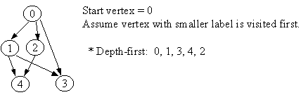
Follow a path until it ends, or until a cycle. Use a stack.

Algorithm:

Let G = (V, E) is a graph which is represented by an adjacency matrix Adj. Assume that nodes in a graph record visited/unvisited information.

procedure DEPTH-FIRST (G)
1. Initialize all vertices as "unvisited".
2. Let S be a stack.
3. Push the root on S.
4. While S not empty, do
5.   begin
6.   Let n <- Pop S.
7    If n is marked as "unvisited", then
8.     begin
9.     Mark n as "visited", and output n to the terminal.
10.     For each vertex v in Adj[n], do
11.       If v is marked as "unvisited", then // this test is actually redundant
12.         push v on S.
13.    end
14.  end

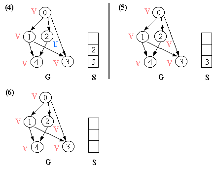
8.2 Breadth-First Traversal

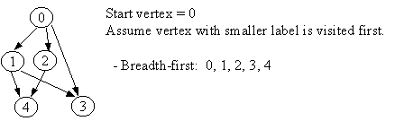
Visit nodes layer-by-layer. Use a queue.

Algorithm :

procedure BREADTH-FIRST (G) 1. Initialize all vertices as "unvisited". 2. Let Q be a queue. 3. Enqueue the root on Q. 4. While Q not empty, do 5. begin 6. n <- Dequeue Q. 7. If n is marked as "unvisited", then 8. begin 9. Mark n as "visited", and output n to the terminal. 10. For each vertex v in Adj[n], do 11. If v is marked "unvisited", then 12. enqueue v on Q.

13. end 14. end

9. Graph Search

Two search methods corresponding to the two traversal schemes above: Depth-First Search (DFS) and Breadth-First Search (BFS).
Terminate search/traversal as soon as the item is found.

10. Minimum Spanning Trees (MST)

A minimum spanning tree T of an undirected graph G is a subgraph of G that connects all the vertices in G at the lowest total cost.
MST is used as one of the most important tools to analyze computer networks (e.g. cabling, network load capacity, optimal flow).
Two algorithms: Prim's algorithm and Kruskal's algorithm.
They are both greedy algorithms.

10.1 Prim's Algorithm

Maintains ONE TREE throughout the algorithm, and make it grow by adding edge by edge.
The idea is to select the next edge
- which is adjacent from any vertex/node in the tree built so far; and
- which has the lowest weight among alternatives (i.e., all edges connected from any vertex/node in the tree built so far).

Algorithm:

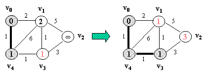
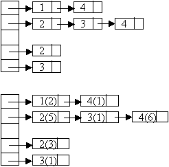
Let G = (V, E) which is represented by an adjacency list Adj. Some support data structures:

d is an array of size |V|. Each d[i] contains the shortest distance for vertex i
Q is a priority queue of UNKNOWN vertices.
p is an array of size |V|. Each P[i] contains the parent of vertex i.
s is the source vertex.

PRIM(G, s)
1. Initialize d[s] with 0, P[s] with 0, and
    all other d[i] (i!=s) with a positive infinity and
              p[i] (i!=s) with 0.
2. Q <- V  // initialize Q with all vertices as UNKNOWN
3. while Q not empty do
4.   begin
5.   u <- ExtractMin(Q)  // Q is modified
6.   Mark u as KNOWN     // Dequeing u is the same as marking it as KNOWN
7.   for each vertex v in Adj[u] do
8.     begin
9.     if v is UNKNOWN and d[v] > weight(u, v), then do
10.      begin
11.      d[v] = weight(u, v)  // update with shorter weight
12.      p[v] = u             // update v's parent as v
13.      end
14.    end
15.  end

Example (NOTE: v0 is the source vertex, and d[i] for each vertex i is also indicated in its circle):

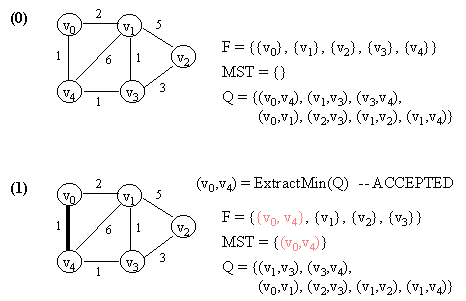
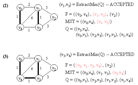
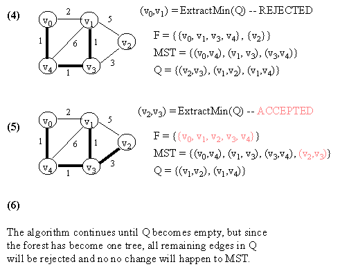
10.2 Kruskal's Algorithm

The main idea is to
- start with a set (called forest) of singleton trees, and
- merge two trees at a time, unless it creates a cycle in the merged tree, until the forest becomes one tree.
The algorithm makes use of notions such as forest and union-find algorithm. But even without knowing them, you can intuitively understand Kruskal's algorithm quite easily.

Algorithm:

Let G = (V, E) which is represented by an adjacency list Adj. Some support data structures:

F is the forest -- a set of all (partial) trees.
MST is the minimum spanning tree, represented by a set of edges.
Q is a priority queue of edges.

KRUSKAL(G)
1. Let F be a set of singleton set of all vertices in G.
2. MST <- {}
3. Q <- E
4. while Q not empty do
5.   (u, v) <- ExtractMin(Q)            // Q is modified
6.   if FIND-SET(u) != FIND-SET(v) then // FIND-SET(i) returns the set in F
                                        // which vertex i belongs to.
                                        // This effectively does cycle check.
                                        // If ACCEPTED,
7.     begin
8.     merge(FIND-SET(u),FIND-SET(v)) in F
9.     MST <- MST Union {(u, v)}
10.    end
11. return MST.

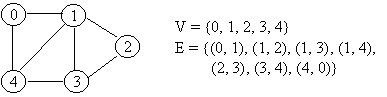
NOTE: In the figure below, a number in a vertex indicates the vertex number (NOT any kind of value).

Graphs

1. Basic definitions

2. Graph Representations

3. Theorem :

4. Simple Graph :

5. Isomorphisms of Graphs

6. Planar Graph

7. Dijkstra's Shortest-Path Algorithm

8. Graph Traversal

9. Graph Search

10. Minimum Spanning Trees (MST)

Some other links to the related graph topics :